rleafmap
Interactive cartography with R and Leaflet
INRA, UMR CARRTEL
75 avenue de Corzent
74200 Thonon-les-Bains
francois.keck@thonon.inra.fr
![]() @FrancoisKeck
@FrancoisKeck
[It is recommended to change your browser to fullscreen (F11) to prevent display problems]
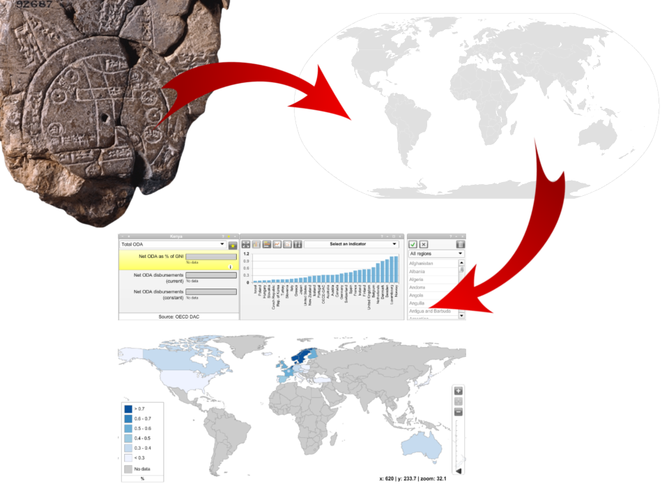
Added values of interactive maps
Multi-scales maps
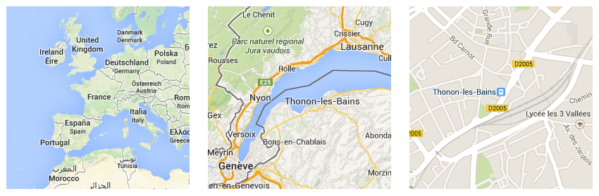
e.g. Google Maps
20 scale levels from 1:590.000.000 to 1:1000.
Slippy maps
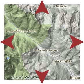
To work on large areas with small scale
You need 250.000 maps 1:25.000 to represent world's total land surfaces
Displaying and handling data
- Multiple and independent data layers
- Combine several maps into one
- Users can be editors
Multimedia and Hypermedia
- The map can support other media (text, pictures, videos...)
- The map is part of the hypertext network
Interactive maps with R
It already exists!
Some packages : googleVis, plotGoogleMaps, rMaps, leafletR, webmaps...
Based on different techniques :
SVG format, Google Chart, Google Maps API, Leaflet, OpenLayers...
rleafmap = R + Leaflet
rleafmap is an R package
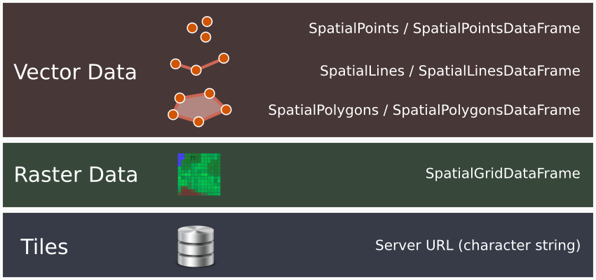
It is designed to export data that inherit the Spatial* class (sp package, Bivand et al. 2008) to a Leaflet interactive map
rleafmap is available here: www.francoiskeck.fr/rleafmap/
install.packages("~/rleafmap_0.1.tar.gz", repos = NULL, type = "source")

library(sp)
library(rleafmap)
Leaflet
rleafmap works with Leaflet, an open-source JavaScript library for web-mapping created by Vladimir Agafonkin.
Some advantages
- Leaflet is light (33kb)
- Leaflet is easy to learn
- Leaflet is mobile-friendly
Supported data
Basic operations
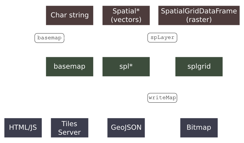
The writeMap function
writeMap(...,
			dir = getwd(),
			prefix = "",
			width = 700, height = 400,
			setView = c(0,0),
			setZoom = 6,
			interface = NULL,
			lightjson = FALSE,
			directView = c("viewer", "browser", "disabled"),
			leaflet.loc = "online")
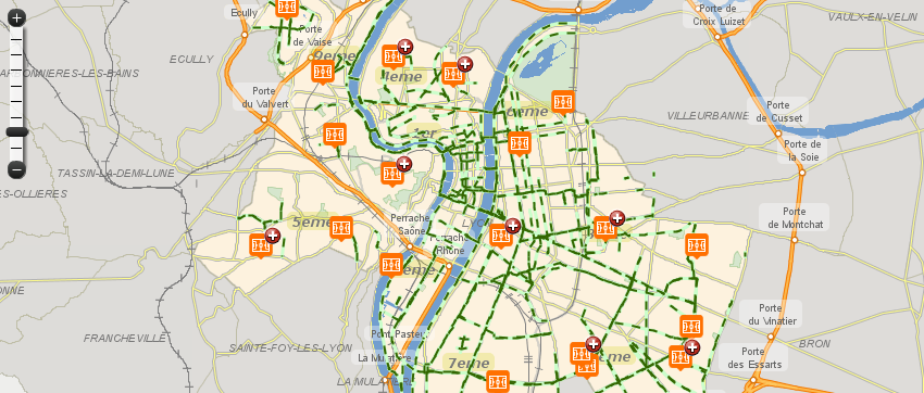
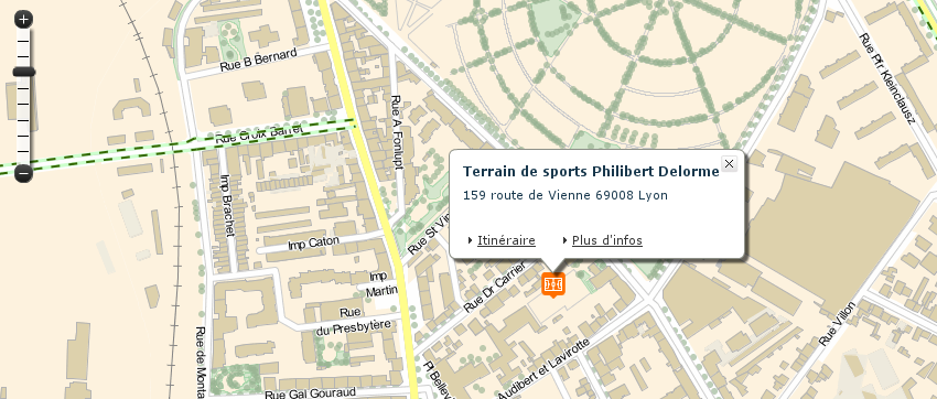
First example
Bicycle sharing system in Lyon (Velo'v stations)
library(sp)
velov <- read.table("velov.txt", h = T)
coordinates(velov) <- ~lon+lat

library(rleafmap)
stamen.toner <- basemap("stamen.toner")
velov.map <- spLayer(velov, stroke = F, popup = velov$stations.name)
writeMap(stamen.toner, velov.map, setView = c(45.76, 4.85), setZoom = 12)
First example
Bicycle sharing system in Lyon (Velo'v stations)
The basemap function
Use basemap() to easily create a new tiles layer (tiles are downloaded from a web server)
A list of pre-configured server is provided
- mapquest.map
- mapquest.sat
- stamen.toner (+ variations)
- stamen.watercolor
But any valid tiles server URL can be used
basemap("stamen.toner")
basemap("stamen.watercolor")
#User defined server: Mapbox Tiles example
basemap("https://a.tiles.mapbox.com/v3/examples.map-i875mjb7/{z}/{x}/{y}.png")
#User defined server: Mapbox Eleanor Lutz "Space Station"
basemap("https://a.tiles.mapbox.com/v3/eleanor.ipncow29/{z}/{x}/{y}.png")
The spLayer() function
The generic function spLayer() allows to create a new data layer (vector or raster)
A set of arguments can be used to customize the way data are displayed
- size
- png, png.width, png.height
- stroke, stroke.col, stroke.lwd, stroke.lty, stroke.alpha
- fill, fill.col, fill.alpha
- cells.col, cells.alpha
The popup argument can be used to add contextual informations d'info-bulles
spLayer - Polygons
French camp sites distribution
data(campsites)

gcol <- rev(heat.colors(5))
gcut <- cut(campsites$N.CAMPSITES, breaks = c(-1, 20, 40, 60, 80, 1000))

pop <- paste(campsites$DEP.NAME, " (", campsites$DEP.CODE, ")
",
             campsites$N.1, "★
", campsites$N.2, "★★
",
             campsites$N.3, "★★★
", campsites$N.4, "★★★★
",
             campsites$N.5, "★★★★★", sep = "")

cs <- spLayer(campsites, fill.col = gcol[as.numeric(gcut)], popup = pop)
writeMap(mq.map, cs, setView = c(46.5, 3), setZoom = 5)
spLayer - Polygons
French camp sites distribution
spLayer - raster heatmap
Vélo'v stations density
library(spatstat)
win <- owin(xrange = bbox(velov)[1,] + c(-0.01,0.01),
            yrange = bbox(velov)[2,] + c(-0.01,0.01))
velov.ppp <- ppp(coordinates(velov)[,1], coordinates(velov)[,2], window = win)
velov.ppp.den <- density(velov.ppp, sigma = 0.005)
velov.den <- as.SpatialGridDataFrame.im(velov.ppp.den)
velov.den$v[velov.den$v < 10^3] <- NA

velov.d <-spLayer(velov.den, layer = "v",
                  cells.alpha = seq(0.1, 0.8, length.out = 12))
writeMap(mapbox, velov.d, setView=c(45.76, 4.85), setZoom = 12)
spLayer - raster heatmap
Vélo'v stations density
The ui() function
The ui() function allows to customize the user interface
ui(zoom = c("topleft", "topright", "bottomleft", "bottomright", "none"),
   layers = c("none", "topright", "topleft", "bottomleft", "bottomright"),
   attrib = c("bottomright", "topleft", "topright", "bottomleft", "none"),
   attrib.text = "")
The layers argument can be used to add a layer selector
A multi-layered map
Vélo'v stations + Vélo'v stations density + Bicycle lanes
vcycle <- readShapeLines("amenagement_cyclable")
vcycle.map <- spLayer(vcycle, stroke.col = "red", stroke.lwd = 1.3,
                      stroke.lty = c(5,3))

velov.ui <- ui(layers = "topright")

writeMap(stamen.toner, mapbox.terrain, velov.d, velov.map, vcycle.map,
         interface = velov.ui, setView = c(45.76, 4.85), setZoom = 13)
A multi-layered map
Vélo'v stations + Vélo'v stations density + Bicycle lanes
RStudio integration
writeMap(..., directView = "viewer")
RStudio Integration
writeMap(..., directView = "viewer")